If you examine the graph you made in the performance evaluation, you may be unpleasantly surprised by your program's performance. Alternatively, you may be quite pleased with your program's performance, but your boss or your dissertation committee want to know how you got such good results. It may be unclear as to what exactly is going on. In order to clarify things, you will want to perform a least-squares fit of your data (performance timings) to an equation that models the performance of your code.
There are three main categories into which everything that your program does will fit: communication, computation, and idle/serial. These categories are mostly self-explanatory. When you are sending and receiving data, that falls into the communication category; when you are crunching numbers, that falls into the computation category; and when one processor is doing an inherently serial operation, or when a processor is waiting for others to finish, then these actions are in the idle/serial category. We can classify each major piece of the algorithm into one of the three categories, and use this information to develop an equation that models the performance of our parallel program.
Suppose we had written a program that finds the numerical integral of a program using Monte Carlo quadrature. The idea of Monte Carlo quadrature is that we can approximate the area under a curve (in 1-D) or the volume under a surface (in 2-D) or the hypervolume under a hypersurface (in n-D) as a function of the average value of the function sampled over the problem domain. In math notation, that's ∫V f(x) dV = V/P ∑i=1P f(xi). The accuracy of the integral is proportional to 1/√P, where P is the number of times we evaluate the function. In order to understand this example, all you really need to know is that we want to compute P different values of the function f(x), and at the end we're going to do something with them.
What follows this paragraph is some C-like pseudocode for this Monte Carlo quadrature program. When I write a program, I generally write out on a piece of paper* a basic algorithm in a code style that is similar to C but that may not be syntactically correct and that may have some commands missing (because I can't remember the exact syntax, or because I don't feel like writing them out). Notes in red are notes to the reader that I would not normally put in my pseudocode. (I also wouldn't put so many comments in my own pseudocode since I mostly know what I'm talking about already.) I recommend writing pseudocode before tackling anything but the simplest of programs.
#include <mpi.h>
#include <stdio.h>
int main(int argc, char **argv) {
// declaration of variables
int me, np;
long P; /* number of function evaluations */
double my_result;
MPI_Status status;
// initialization and environmental inquiry
MPI_Init(&argc, &argv);
MPI_Comm_rank(MPI_COMM_WORLD, &me);
MPI_Comm_size(MPI_COMM_WORLD, &np);
if (me == 0) {
// manager process
// receive input from user as to accuracy we want
double tol;
// tol = input (this is not proper C syntax but I will find the right syntax later)
P = (long) 1./(tol*tol); (the (long) coerces the type, forcing it to go from type double to type long)
long Psend = P/np; // everybody does one npth of the work
for (int i = 1; i < np; i++) {
// send Psend to all worker processors
MPI_Send(&Psend, 1, MPI_LONG, i, me, MPI_COMM_WORLD);
}
// now, do my own Monte Carlo
my_result = monte_carlo(Psend);
double final_result = my_result/np;
for (int i = 1; i < np; i++) {
// receive results from worker processors
double tmp_result;
MPI_Recv(&tmp_result, 1, MPI_DOUBLE, i, i, MPI_COMM_WORLD, &status);
final_result += tmp_result;
}
printf("final result of quadrature, for tol=%g, integral=%g", tol, final_result);
} else {
// worker process
MPI_Recv(&P, 1, MPI_LONG, 0, 0, MPI_COMM_WORLD, &status);
my_result = monte_carlo(P);
my_result /= np;
MPI_Send(&my_result, 1, MPI_DOUBLE, me, me, MPI_COMM_WORLD);
}
return 0;
}
double monte_carlo(long P) {
double answer = 0;
for (long i = 0; i < P; i++) {
// evaluate function at pseudorandom point
// add it divided by P to answer (avoid overflow)
}
return answer;
}
Let's examine this code for the different classes of operations. We could make a table detailing what basic operations occur, which processor performs them, and how many of them take place.
| Compu- tation | Communi- cation | Initialization/ Serial/Idle | Which Processor? (how many times) |
|---|---|---|---|
| MPI_Init, MPI_Comm_rank, MPI_Comm_size | All (1) | ||
| Receive input, compute how much work each processor does | Manager (1) | ||
| MPI_Send | Manager (N) | ||
| MPI_Recv | Workers (1 each) | ||
| monte_carlo | All (1) | ||
| MPI_Send | Workers (1 each) | ||
| MPI_Recv | Manager (N) | ||
| Compute integral (sum results from all processors) | Manager (1) | ||
| MPI_Finalize | All (1) |
The total walltime is the sum of the time spent computing, communicating, and in serial activities. So we could work out a formula that would approximate the performance of the algorithm. Let's start with the computation.
TNcomputation = TNmonte-carlo + TNsum.
We can break this down further, because the time it takes to do the Monte Carlo part of the computation is proportional to the total number of Monte Carlo points (P = 1/tol2) and inversely proportional to the number of processors (N). The amount of time required to perform the sum is insignificant, so we can treat it as a constant. So we have
TNcomputation = P/N tmonte-carlo + tsum
= 1/(N tol2) tmonte-carlo + tsum,
where tmonte-carlo is the amount of time for a single Monte Carlo point to be computed.
As for the communication, we do N sends and then N receives. They are all done sequentially, and it is reasonable to assume that they each take the same amount of time, so
TNcommunication = 2N tcommunication.
The cost of communication is equal to the startup cost plus the bandwidth cost. But since we are dealing with such small messages (a single long or double) we can neglect the bandwith cost, so tcommunication = tstartup.
Finally, the third category takes all remaining operations into consideration.
TNserial = Tinit/finalize + Tserial.
There's actually no way to distinguish between the tasks in this category in terms of time, since they do not vary with N. So our final equation looks like this:
TN = TNcomputation + TNcommunication + TNnon-parallel
= 1/(N tol2) tmonte-carlo + tsum + 2N tstartup + tserial.
We would want to do a strong scaling study to provide some data to which we can fit this equation. We would run the program on different numbers of processors (most conveniently, powers of two), running it at least three times and taking the average run time for each N. Suppose we got the following timings** from our strong scaling study, for tol = 10-4:
| N | Average Wall Time (s) |
|---|---|
| 4 | 30.0 |
| 16 | 15.2 |
| 32 | 7.7 |
| 64 | 3.9 |
| 128 | 2.1 |
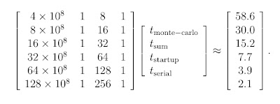
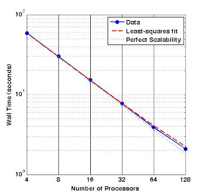
We could make a log-log plot of the results, and see that the algorithm scales pretty well. (You can see this without making a plot by looking at the numbers, and observing that 30.0 is close to one half of 58.6, 15.2 is close to one half of 30.0, etc.) We are not too far off from ideal. The big difference appears to be at the tail end, where the walltime doesn't halve when the processor count is doubled. Let's see how well we can fit these timings to our formula. We have to solve the non-negative least-squares problem

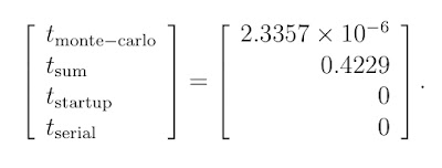
I solved it using Matlab's lsqnonneg function (non-negative least squares), and obtained

We can graph all these results and see how the algorithm performed and how well our function fits the results. The figure shows a log-log plot of number of processors versus walltime. The solid blue line with the blue dots shows the actual performance data. The dashed red line shows our least-squares fit, and the turquoise dotted line shows ideal scaling.

As the number of processors grows, the computation time is not quite halved. We would expect this because the amount of communication is proportional to the number of processors, so doubling the number of processors doubles the amount of communication required. So as the number of processors grows, the amount of work per processor shrinks and the amount of communication per processor grows, and time spent in communication begins to dominate the wall time.
*pre-arm trouble. Nowadays I either minimally sketch it on a piece of paper, or I type pseudocode into a Word document on my laptop and print it out before coding the real thing on my desktop Linux box.
** These numbers were pulled from my posterior. Yes, I totally made them up. Trust me, gubmint auditors, I did not waste valuable computing resources on a blog entry!
Next topic: More on scalability


2 comments:
I liked the example and I think this kind of demonstrations really help explaining were bottlenecks may occur in the parallel code. I would like to add two comments:
1. Solving the matrix and obtaining 0 for the startup time, after already neglecting the bandwidth, means that the problem is totally Embarrassingly Parallel and this is indeed the case for MC calculations. It would be interesting to repeat the exercise for a communication intensive application, e.g. Laplace equation.
2. I think it worth mentioning Collective Communication commands, i.e. Bcast and Reduce in this context. In particular Reduce+Summation can be more efficient than the loop over the Recv because it can do summation out of order and this may hide some of the holding/communication time. Another alternative is to use MPI ANY_SOURCE in the Recv command.
--Guy
Guy, thanks for your comments.
You are absolutely right that this is an embarrassingly parallel calculation and the communication costs are negligible. It would scale quite well to tens of thousands of processors. I agree that a more communication-intensive algorithm would be more interesting to evaluate.
If I were actually writing this code for real, I would absolutely use collective communications (MPI_Bcast and MPI_Reduce). They would be much more efficient because they are usually tree-based algorithms so the work of sending or receiving messages is dispersed. The reason I didn't use them for this example program is that in my mini-course here I introduced only the six basic commands (MPI_Init, MPI_Finalize, MPI_Comm_size, MPI_Comm_rank, MPI_Send, and MPI_Recv), and I didn't want to use anything I hadn't yet covered.
Thanks for bringing up those points!
Post a Comment